The Complete Generative AI Roadmap: Beginner to Pro
A generative ai roadmap is a structured learning path designed to guide software engineers from foundational programming and mathematics through advanced machine learning, deep learning, and transformer architectures. It provides a systematic approach to mastering foundation models, fine-tuning techniques, retrieval-augmented generation (RAG), and model deployment workflows.
The paradigm shift brought about by Generative Artificial Intelligence (GenAI) has fundamentally altered how software systems operate. Rather than relying on rigid, rule-based algorithms or traditional classification models, modern architectures leverage probabilistic generation. This shift requires engineers to understand highly complex neural architectures capable of parsing context, retaining state, and predicting sequential data across multiple modalities, including text, image, and audio.
Mastering GenAI is not simply about learning how to prompt an API. It requires a profound, bottom-up understanding of the underlying mechanics—ranging from calculus and gradient descent to distributed training, low-rank adaptation, and vector-space embeddings. Without a deep comprehension of these internal mechanics, software engineers cannot effectively optimize inference latency, reduce hallucination rates, or fine-tune models to fit domain-specific constraints.
This guide serves as a comprehensive, strictly technical generative AI roadmap. It outlines the exact progression of skills, theoretical frameworks, and implementation paradigms required to transition from foundational computer science principles to deploying production-grade Large Language Models (LLMs) and multi-modal generative systems.
Step 1: Programming and Mathematical Foundations
Before attempting to construct or train neural networks, you must build a robust foundation in the mathematical principles that govern machine learning algorithms and the programming languages used to implement them. Machine learning is fundamentally applied mathematics. Deep learning frameworks abstract away much of the calculus and linear algebra, but a lack of mathematical intuition will severely limit your ability to debug vanishing gradients, optimize learning rates, or understand dimensional mismatches in tensor operations. The prerequisites involve mastering Python—the definitive language of artificial intelligence—and the statistical mathematics required to model probability distributions.
Python Proficiency and Vectorized Computation
Python is the lingua franca of AI due to its extensive ecosystem of scientific computing libraries. Proficiency must extend beyond basic syntax; you must understand memory management, generator functions, and asynchronous execution. More importantly, you must master vectorized operations using NumPy and Pandas. Traditional iterative loops (e.g., for loops) are computationally inefficient for the massive matrix multiplications required in AI.
You must be highly comfortable manipulating multi-dimensional arrays (tensors). Understanding broadcasting, dot products, and matrix transformations natively in NumPy is critical before moving to GPU-accelerated frameworks like PyTorch or TensorFlow.
Linear Algebra
Linear Algebra is the engine of deep learning. Neural networks represent data as multi-dimensional vectors and apply linear transformations followed by non-linear activations. You must understand:
- Scalars, Vectors, Matrices, and Tensors: The hierarchical structures of data representation.
- Matrix Multiplication and Dot Products: The mathematical core of forward propagation.
- Eigenvalues and Eigenvectors: Crucial for understanding dimensionality reduction techniques like Principal Component Analysis (PCA).
- Singular Value Decomposition (SVD): A foundational concept for low-rank approximation, which directly applies to modern parameter-efficient fine-tuning techniques like LoRA.
Multivariate Calculus
Calculus powers the optimization process of neural networks. You must comprehend how models learn through the minimization of a loss function over a high-dimensional surface.
- Partial Derivatives and Gradients: Calculating the rate of change of the loss with respect to individual model weights (∂L/∂W).
- The Chain Rule: The core mathematical theorem that enables Backpropagation, allowing gradients to be calculated backwards through multiple hidden layers.
Probability and Information Theory
Generative models are probabilistic engines. They do not store databases of facts; they approximate data distributions and sample from them.
- Probability Distributions: Normal (Gaussian), Bernoulli, and Binomial distributions.
- Bayes’ Theorem: P(A|B) = P(B|A)P(A) / P(B), foundational for Bayesian inference and understanding conditional probabilities.
- Cross-Entropy and Kullback-Leibler (KL) Divergence: Metrics used to measure the difference between two probability distributions, heavily utilized in loss functions for classification and generative modeling.
Step 2: Core Machine Learning and Deep Learning
Transitioning from theoretical mathematics to applied algorithms involves understanding how machines extract patterns from data. This step requires moving from traditional statistical learning models to deep, non-linear neural networks. Deep learning is the direct predecessor to modern generative AI; understanding the architecture of a Multi-Layer Perceptron (MLP) and how gradients flow through a network is non-negotiable. Modern GenAI frameworks are essentially massive deep learning models scaled across billions of parameters. This stage necessitates writing custom training loops, defining custom loss functions, and managing tensor operations directly on GPUs.
Traditional Machine Learning (Scikit-Learn)
Before jumping to deep learning, understand the classical ML algorithms. This provides a baseline for evaluating whether a complex neural network is actually necessary for a given problem.
- Supervised Learning: Linear Regression, Logistic Regression, Support Vector Machines (SVM), and Random Forests.
- Unsupervised Learning: K-Means Clustering, DBSCAN, and PCA.
- Evaluation Metrics: Precision, Recall, F1-Score, and the Area Under the Receiver Operating Characteristic Curve (ROC-AUC).
Neural Networks and Deep Learning Fundamentals (PyTorch)
Deep learning replaces manual feature engineering with hierarchical feature extraction. PyTorch is the industry-standard framework due to its dynamic computational graph (autograd).
- Perceptrons and MLPs: The fundamental building blocks consisting of input layers, hidden layers, and output layers.
- Activation Functions: Introducing non-linearity into the network. You must understand the mathematical mechanics and use cases for ReLU, GeLU, Sigmoid, and Softmax.
- Loss Functions: Mean Squared Error (MSE) for regression and Cross-Entropy Loss for multi-class classification.
- Optimizers: Stochastic Gradient Descent (SGD) and Adam (Adaptive Moment Estimation). The weight update rule is defined as: θnew = θold – α∇J(θ), where α is the learning rate and ∇J(θ) is the gradient of the loss function.
import torch
import torch.nn as nn

# Example of a simple Feed-Forward Neural Network in PyTorch
class SimpleNN(nn.Module):
    def __init__(self, input_size, hidden_size, num_classes):
        super(SimpleNN, self).__init__()
        self.fc1 = nn.Linear(input_size, hidden_size)
        self.relu = nn.ReLU()
        self.fc2 = nn.Linear(hidden_size, num_classes)

    def forward(self, x):
        out = self.fc1(x)
        out = self.relu(out)
        out = self.fc2(out)
        return out
Step 3: Natural Language Processing (NLP) Foundations
Natural Language Processing bridges the gap between raw human language and numerical tensor representations. Because machine learning models can only process numbers, text must be systematically broken down, mapped to discrete integers, and eventually projected into continuous, high-dimensional vector spaces. A thorough understanding of legacy NLP techniques provides crucial context for why modern architectures are designed the way they are. You must understand the limitations of sequential processing and the necessity of semantic embeddings before progressing to Large Language Models.
Tokenization
Tokenization is the process of splitting raw text into manageable sub-units (tokens). Modern GenAI models do not process character-by-character or word-by-word.
- Byte-Pair Encoding (BPE): A subword tokenization algorithm used by GPT models that merges the most frequently occurring byte pairs iteratively.
- WordPiece: Used by BERT, similar to BPE but maximizes the likelihood of the training data rather than relying strictly on frequency.
Word Embeddings
Embeddings project tokens into a dense vector space where semantic similarity is represented by spatial proximity.
- Word2Vec and GloVe: Early embedding models that mapped words to fixed-dimensional vectors. If two words are used in similar contexts, their vectors will have a high cosine similarity.
- Limitation: These are static embeddings. The word “bank” (financial institution) and “bank” (river edge) share the exact same vector in Word2Vec, ignoring context.
Sequence Models (RNNs, LSTMs, GRUs)
Prior to Transformers, Recurrent Neural Networks (RNNs) were the standard for sequential data.
- RNN Architecture: Processes tokens sequentially, updating a hidden state vector at each step.
- The Vanishing Gradient Problem: Standard RNNs struggle to retain information from early in the sequence due to gradients exponentially shrinking during backpropagation through time (BPTT).
- LSTMs (Long Short-Term Memory): Introduced gating mechanisms (Forget, Input, Output gates) to regulate the flow of information and maintain long-term dependencies.
Step 4: The Transformer Architecture (The Core of GenAI)
The publication of the “Attention Is All You Need” paper by Vaswani et al. in 2017 triggered the current Generative AI revolution. The Transformer architecture entirely discarded recurrence (RNNs/LSTMs) in favor of the Self-Attention mechanism, enabling massive parallelization during training and significantly deeper context windows. Understanding the Transformer at a granular, mathematical level is the single most important milestone in this generative ai roadmap. You must comprehend how queries, keys, and values interact, how positional information is injected into order-agnostic architectures, and how multi-head attention captures diverse linguistic nuances.
The Self-Attention Mechanism
Self-attention allows the model to weigh the importance of every token in a sequence relative to every other token, simultaneously.
For each token, the network generates three vectors via learned linear transformations:
- Query (Q): What the current token is looking for.
- Key (K): What the token is offering to other tokens.
- Value (V): The actual semantic content of the token.
The Scaled Dot-Product Attention is calculated as:
Attention(Q, K, V) = Softmax((Q Kᵀ) / √dₖ) V
The dot product of Q and Kᵀ yields attention scores. Dividing by √dₖ (the square root of the dimension of the key vectors) scales the values to prevent gradients from disappearing during the Softmax operation. The resulting probabilities are multiplied by V to create a context-aware vector representation.
Multi-Head Attention
Instead of performing a single attention function, Transformers project Q, K, and V multiple times into lower-dimensional spaces, compute attention independently for each “head”, and concatenate the results. This allows the model to jointly attend to information from different representation subspaces (e.g., one head tracking grammatical structure, another tracking semantic entity relationships).
Positional Encoding
Because Transformers process all tokens simultaneously (in parallel) rather than sequentially, they inherently lack the concept of sequence order. Positional encodings—typically generated using alternating sine and cosine functions of different frequencies—are added to the input embeddings at the bottom of the encoder and decoder stacks to inject absolute and relative positional context.
Step 5: Large Language Models (LLMs) and Foundation Models
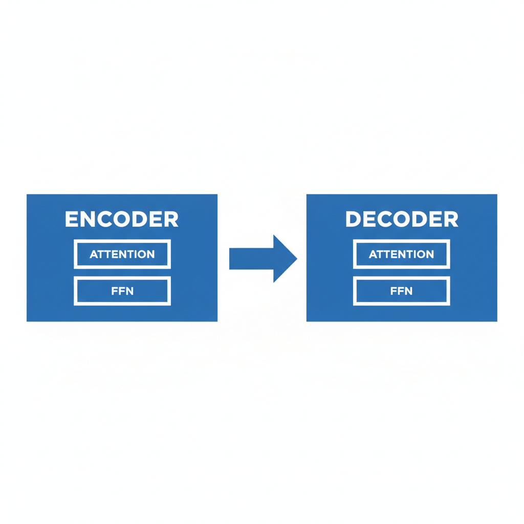
Once the underlying Transformer architecture is mastered, the next phase involves understanding how these structures are scaled to billions of parameters to create Foundation Models. These are massive probabilistic models trained on internet-scale corpora using self-supervised learning objectives. The distinction between different LLMs often lies in their architectural focus: some utilize only the Encoder block of the Transformer, some use only the Decoder, and others utilize both. Understanding these structural paradigms dictates which model is appropriate for specific downstream engineering tasks, such as text generation, sentiment classification, or code translation.
Architectural Paradigms
- Encoder-Only Models (e.g., BERT, RoBERTa): Utilize bidirectional context to understand the relationships between words. They are heavily optimized for Natural Language Understanding (NLU) tasks like classification, named entity recognition (NER), and extractive question answering. They are trained via Masked Language Modeling (MLM).
- Decoder-Only Models (e.g., GPT-3/4, LLaMA, Mistral): Highly optimized for Natural Language Generation (NLG). They operate strictly autoregressively, predicting the next token in a sequence based only on preceding tokens (unidirectional context).
- Encoder-Decoder Models (e.g., T5, BART): Utilize both blocks. Highly effective for sequence-to-sequence tasks such as language translation and text summarization.
The Training Pipeline
- Pre-Training: The computationally massive phase where the model learns raw language statistics and world knowledge from trillions of tokens.
- Supervised Fine-Tuning (SFT): Training the base model on high-quality instruction-response pairs to teach it how to follow user commands.
- Alignment (RLHF/DPO): Aligning the model with human preferences to ensure the output is helpful, honest, and harmless, often utilizing Reinforcement Learning from Human Feedback (RLHF) or Direct Preference Optimization (DPO).
Step 6: Advanced Customization: Fine-Tuning and PEFT
Foundation models are general-purpose. To engineer solutions for highly specific enterprise use cases (e.g., medical diagnostics, legal contract review), you must customize the model’s behavior and knowledge. Full-parameter fine-tuning—updating every weight in an LLM—is computationally prohibitive for models with billions of parameters, often requiring massive clusters of A100 or H100 GPUs. Consequently, Parameter-Efficient Fine-Tuning (PEFT) has become the industry standard for adapting LLMs efficiently. You must understand the mathematical tricks used to inject domain-specific capabilities into models while freezing the vast majority of their original architecture.
LoRA (Low-Rank Adaptation)
LoRA bypasses the need to update the massive weight matrices of an LLM. Instead of updating a pre-trained weight matrix W₀, LoRA freezes W₀ and injects trainable rank decomposition matrices A and B.
The updated weights are represented mathematically as: W = W₀ + ∆W = W₀ + B A
If W₀ is a 4096 x 4096 matrix, a full update requires ~16.7 million parameters. By setting a low rank (e.g., r = 8), matrix A becomes 4096 x 8, and matrix B becomes 8 x 4096. The total trainable parameters drop to ~65,000, drastically reducing VRAM requirements and allowing fine-tuning on consumer-grade hardware.
QLoRA (Quantized LoRA)
QLoRA takes LoRA a step further by quantizing the base model weights (W₀) down to 4-bit precision (NormalFloat4) while maintaining the adapters (A and B) in 16-bit precision. This allows a 65-billion parameter model to be fine-tuned on a single 48GB GPU without significant degradation in performance.
Step 7: Retrieval-Augmented Generation (RAG) and Vector Databases
Large Language Models suffer from several systemic limitations: their knowledge is frozen in time at the end of their pre-training run, they lack access to proprietary enterprise data, and they are prone to “hallucinations” (generating plausible but factually incorrect information). Retrieval-Augmented Generation (RAG) addresses these flaws by coupling the generative power of an LLM with external data retrieval mechanisms. Understanding RAG architecture is paramount for software engineers building production-grade enterprise applications. It requires mastering semantic search, chunking strategies, and vector-space geometry.
The RAG Pipeline
- Ingestion and Chunking: Proprietary documents (PDFs, Confluence pages) are parsed and split into overlapping textual chunks to preserve context while adhering to token limits.
- Embedding Generation: An embedding model (e.g., text-embedding-ada-002) converts these chunks into dense vector representations.
- Vector Database Storage: The vectors, alongside their metadata, are indexed in a specialized Vector Database (e.g., Pinecone, ChromaDB, Milvus, Qdrant).
- Retrieval via Cosine Similarity: When a user submits a prompt, the prompt is embedded into a vector. The system calculates the distance between the prompt vector and the document vectors in the database. The mathematical formulation for Cosine Similarity is: (A · B) / (||A|| ||B||).
- Augmented Generation: The top-k most relevant text chunks are appended to the user’s prompt as context, and the LLM synthesizes an accurate answer grounded strictly in the retrieved data.
Advanced RAG Techniques
Basic RAG pipelines fail in complex scenarios. Advanced architectures require implementing techniques such as Query Expansion, HyDE (Hypothetical Document Embeddings), Parent-Child Chunking, and Re-ranking models (e.g., Cohere Re-rank) to surface the most contextually relevant information.
Step 8: Multi-Modal AI and Image Generation
The scope of Generative AI extends far beyond text. Modern systems parse and generate cross-modal data, linking natural language to images, video, and audio. To build fully comprehensive GenAI systems, you must understand the entirely different mathematical paradigms that drive visual generation. Unlike autoregressive Transformers, image generation predominantly relies on stochastic differential equations and continuous noise processes. A complete generative ai roadmap must cover both Diffusion models and Generative Adversarial Networks.
Diffusion Models
Diffusion models (e.g., Stable Diffusion, Midjourney) learn to generate images by reversing a gradual noise-addition process.
- Forward Diffusion (Markov Chain): Gaussian noise is iteratively added to a high-resolution image over hundreds of steps until it becomes pure, unrecognizable static noise.
- Reverse Diffusion: A U-Net architecture, conditioned on text embeddings (e.g., from CLIP), learns to iteratively denoise the image, predicting the noise added at each step and subtracting it to reveal a coherent structure.
- Latent Diffusion: To optimize computational efficiency, Stable Diffusion does not operate in high-dimensional pixel space. Instead, it compresses images into a lower-dimensional “latent space” using an Autoencoder, applies the diffusion process, and decodes the result back into an image.
Generative Adversarial Networks (GANs)
Though largely superseded by Diffusion models for pure image synthesis, GANs remain highly relevant for real-time generation, video upscaling, and domain translation (e.g., changing day to night in a video). GANs operate on a min-max game theory framework involving two neural networks:
- The Generator: Attempts to create fake data that is indistinguishable from real data.
- The Discriminator: Acts as a binary classifier, attempting to distinguish between real data and the Generator’s fake data.
The networks train simultaneously, forcing each other to improve until the Generator produces highly realistic outputs.
Step 9: LLMOps and Deployment Optimization
Training a model is only half the battle; deploying massive neural networks efficiently to production environments is a severe engineering challenge. LLMOps (Large Language Model Operations) encompasses the deployment, monitoring, and orchestration of GenAI models at scale. Engineers must contend with high latency, massive GPU memory constraints, and continuous prompt management. This stage transitions a data science prototype into a scalable, highly concurrent microservice infrastructure.
Model Quantization and Serving
To run large models efficiently, weights must be compressed (Quantization) with minimal loss of accuracy. Techniques like Post-Training Quantization (PTQ) and Activation-Aware Weight Quantization (AWQ) map high-precision floats (FP16) to lower-precision integers (INT8 or INT4).
Serving engines like vLLM and Triton Inference Server utilize techniques such as Continuous Batching and PagedAttention (which manages K-V cache memory like an operating system manages virtual memory) to maximize throughput and minimize Time to First Token (TTFT).
Orchestration Frameworks
Developing robust agentic workflows requires orchestration libraries that handle state management, API tool calling, and chaining complex logic.
- LangChain: Provides abstractions for chaining prompts, memory modules, and agents capable of taking actions based on LLM reasoning.
- LlamaIndex: Specialized strictly for deep data ingestion, advanced RAG architectures, and complex querying pipelines over proprietary datasets.
Comparison: RAG vs. Fine-Tuning
A critical architectural decision for engineers is choosing between RAG and Fine-Tuning when adapting an LLM. They are not mutually exclusive; they serve fundamentally different purposes and are often used in tandem.
| Feature / Characteristic | Retrieval-Augmented Generation (RAG) | Fine-Tuning (PEFT / LoRA) |
|---|---|---|
| Primary Use Case | Injecting dynamic, real-time, or proprietary data into the model’s context. | Teaching the model new behaviors, specific tones, or domain-specific logic and syntax. |
| Knowledge Updates | Instantaneous. Simply update the Vector Database; no retraining required. | Static. Requires another training loop and dataset curation to update facts. |
| Hallucination Mitigation | Highly effective. Responses are directly grounded in retrieved document chunks. | Moderate. The model can still hallucinate information outside its training distribution. |
| Computational Cost | Low. Requires vector embeddings and database queries. | High. Requires GPUs to compute gradients and update model weights. |
| Data Privacy | High. Sensitive data remains in the vector store and is injected only when necessary. | Variable. Private data is baked into the model weights, risking data extraction attacks. |
Frequently Asked Questions (FAQ)
How long does it take to complete a generative ai roadmap?
For a developer already proficient in Python, mastering the fundamental mathematics, deep learning frameworks (PyTorch), and Transformer architecture typically requires 3 to 6 months of intensive study. Transitioning to advanced topics like LoRA fine-tuning, complex RAG pipelines, and LLMOps can take an additional 6 to 12 months of practical, project-based engineering.
Do I need to buy expensive GPUs to learn Generative AI?
No. While training large models from scratch requires massive enterprise compute, learning and executing PEFT (like QLoRA) or building RAG pipelines can be done using cloud-based notebooks (Google Colab, Kaggle) which provide free access to T4 or P100 GPUs. Additionally, local inference of quantized models is highly achievable on consumer hardware using tools like Ollama or LM Studio.
What is the difference between AI, ML, Deep Learning, and Generative AI?
Artificial Intelligence (AI) is the broad concept of machines simulating human intelligence. Machine Learning (ML) is a subset of AI involving algorithms that learn from data without explicit programming. Deep Learning (DL) is a subset of ML using multi-layered neural networks to extract complex features. Generative AI is a subset of Deep Learning focused specifically on models that create net-new data (text, images, code) rather than just predicting or classifying existing data.
Is LangChain strictly necessary for building GenAI applications?
No. LangChain is an abstraction layer that simplifies the development of complex LLM chains and agents. However, many enterprise teams prefer writing custom code using the official SDKs (like the OpenAI Python SDK or Anthropic SDK) to maintain tighter control over the execution flow, reduce dependency bloat, and optimize performance for specific use cases.